
There is a moment that changes how you think about monitoring forever.
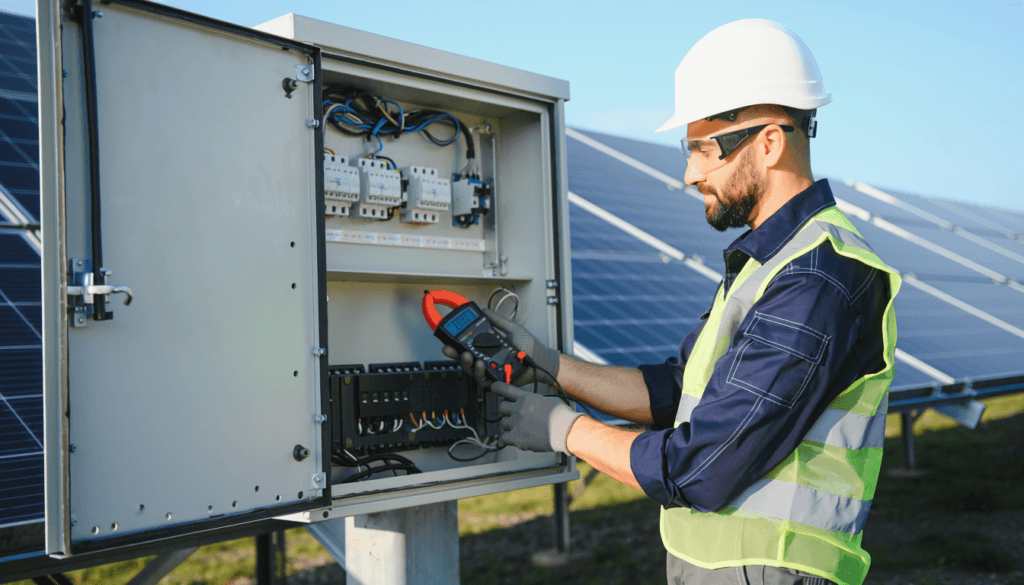
It happens when you walk a site with a current clamp meter — systematically measuring each string at the combiner box level — and find a string producing 15% less than it should. Not 1%. Not 2%. Fifteen percent. A sustained, structural performance gap that has been silently eroding production since commissioning.
You go back to the monitoring system. You look at the historical data for that string. No alerts. No anomalies. No flags of any kind.
The monitoring system did not miss this loss because it malfunctioned. It missed it because of something more fundamental — and more important to understand if you want to actually supervise an industrial solar installation rather than simply observe it.
Disclosure: This article contains affiliate links. If you purchase through these links, I may earn a small commission at no extra cost to you. I only recommend technical resources that I consider genuinely useful for industrial solar professionals working in Africa and the MENA region.
What String Monitoring Actually Measures — And What It Cannot
This is the technical distinction that most O&M training materials gloss over — and that most monitoring vendors have little incentive to explain clearly.
A string monitoring system measures electrical output — voltage, current, and power — at the inverter input level or at combiner box level, depending on the system architecture. It compares this output against expected values, and flags deviations that exceed a configured threshold.
The threshold is the key word. String monitoring systems are designed to detect significant, sudden anomalies — a string that drops to zero, a fuse that blows, an inverter that trips. They are not designed to detect gradual, progressive degradation that stays within the noise band of normal operational variability.
Here is why this matters in practice. A string that degrades from 100% to 85% of expected output over six months does not produce a step-change anomaly that a monitoring system can clearly identify. It produces a slow drift that is consistently masked by three variables that affect every string on every installation every day.
Irradiance variability
Even with irradiance correction applied, the natural variability of solar resource across a day and between days creates a noise band that easily absorbs a 5% to 10% performance gap. A string producing 87% of expected output on a variable irradiance day looks almost identical to a string producing 100% of expected output on a slightly lower irradiance day.
Temperature effects
Panel output varies with temperature according to the temperature coefficient of the module — typically around -0.35% per degree Celsius above 25°C for monocrystalline panels. A string running slightly hotter than neighboring strings — due to partial shading, soiling concentration, or micro-environmental differences — will naturally produce less, and this thermal difference is almost always within the noise band of a monitoring system’s alert threshold.
Soiling non-uniformity
Soiling does not accumulate uniformly across a solar array. Strings near access roads, near industrial exhaust points, or in areas of higher wind deposition accumulate soiling faster than neighboring strings. A monitoring system sees lower output — but without a soiling-corrected baseline for each individual string, it cannot distinguish between normal soiling variation and structural underperformance.
The result is that string losses of 10% to 15% — losses that are financially significant and structurally persistent — routinely fall below the detection threshold of monitoring systems and generate no alerts for months or years.
The Three Types of String Losses That Monitoring Consistently Misses
Understanding why monitoring misses certain losses requires understanding the physical mechanisms behind those losses — because each mechanism has a different detection signature and a different physical inspection method.
Type 1 — Progressive cell degradation and micro-crack propagation
Monocrystalline solar cells degrade over time through a combination of mechanisms — light-induced degradation in the first year, potential-induced degradation driven by voltage stress, and physical micro-cracking caused by mechanical stress from wind loading, thermal cycling, and installation handling.
Micro-crack propagation is particularly relevant to industrial sites in MENA and Africa, where thermal cycling is aggressive — large daily temperature swings between cool nights and hot days create repeated expansion and contraction cycles that stress cell interconnects and propagate micro-cracks that were present but dormant from manufacturing.
The degradation from micro-cracks is gradual, spatially distributed across a string, and presents as a slow decline in short-circuit current and fill factor. A monitoring system sees slightly lower power output — within normal variability. A thermal imaging inspection sees the characteristic hot spots that indicate cell-level electrical resistance increases.
Type 2 — Connection resistance degradation at the string level
DC connections — MC4 connectors, junction box terminals, combiner box connections — degrade over time through oxidation, thermal cycling, and mechanical vibration. Increased connection resistance reduces current flow and generates heat at the point of resistance, without producing a clean open-circuit fault that would trigger a monitoring alert.
A string with significantly degraded MC4 connections at multiple points might show a 5% to 12% reduction in output — distributed across many individual resistance increases that no single monitoring point can isolate.
Type 3 — Partial shading from unplanned obstructions
Partial shading events — from vegetation growth, structure modifications, new equipment installations, or construction activity near the array — reduce string output in ways that are highly variable by time of day and season. A monitoring system sees lower output at certain times but may average this into acceptable daily production totals.
More importantly, the bypass diode behavior in shaded modules creates characteristic current-voltage signatures that are visible in I-V curve tracing but invisible to standard monitoring current measurements.
Summary — Three Loss Types and Their Detection Methods
| Loss Type | Physical Mechanism | Monitoring Signal | Detection Method |
|---|---|---|---|
| Progressive cell degradation | Micro-cracks, PID, light-induced degradation | None — within noise band | Infrared thermography |
| Connection resistance degradation | MC4 oxidation, terminal corrosion | None — distributed across string | Thermal imaging + MC4 pull-test |
| Unplanned partial shading | New obstructions near array | Variable by time of day | I-V curve tracing + visual inspection |
This table is the practical takeaway from years of field observation: every significant string loss has a physical cause, every physical cause has a detection method, and none of those detection methods is a monitoring dashboard alert.
What Physical Inspection Actually Finds — Step by Step
This is the practical protocol used on an industrial installation in Morocco to identify the 15%+ string loss that monitoring never flagged.
Step 1 — Baseline calculation
Before measuring anything on site, calculate the expected string current for current irradiance and temperature conditions. This requires a calibrated reference cell or irradiance sensor giving real-time plane-of-array irradiance, the short-circuit current specification of the panel at STC, and the temperature correction factor based on measured cell temperature or ambient temperature plus a thermal offset.
A practical and cost-effective option for field use is a handheld irradiance meter — such as a calibrated reference cell connected to a digital multimeter. On installations without a dedicated plane-of-array sensor, a reference cell placed at the same tilt and orientation as the array and measured simultaneously with each string provides a reliable irradiance correction baseline that costs under 200 USD to implement.
This corrected baseline is what every measured string current is compared against. Without it, you are measuring numbers without context.
Step 2 — String current measurement at the combiner box
Using a calibrated DC clamp meter — a Fluke 376 FC or equivalent, capable of accurate measurement at the current levels of a standard string (typically 10 to 18 amperes for 580 Wp monocrystalline panels) — measure the current of each string individually at the combiner box terminals.
Record the measured value, the expected value for current conditions, and the deviation percentage. Do this for every string in sequence. The measurement itself takes approximately 30 to 60 seconds per string.
Step 3 — Flag deviations above threshold
Any string showing a deviation greater than 5% from the irradiance and temperature-corrected expected value deserves closer investigation. A deviation above 10% requires immediate follow-up. A deviation above 15% — as found on this installation — represents a financially significant loss that should be treated as a priority corrective action.
Step 4 — Thermal imaging on flagged strings
For each string that shows a significant current deviation, a thermal imaging inspection of the string’s panels identifies hot spots — cell-level anomalies, bypass diode activation patterns, and connection resistance issues — that give the physical cause of the electrical deviation. This step requires an IR camera and should be performed under stable, high-irradiance conditions, ideally between 10 AM and 2 PM.
Step 5 — MC4 connector inspection and I-V curve tracing
For strings where thermal imaging does not clearly identify the cause of the deviation, manual inspection of MC4 connectors and junction box terminals — combined with I-V curve tracing using a portable curve tracer — provides the additional diagnostic resolution needed to distinguish between connection degradation, cell degradation, and shading effects.
The Financial Case for a Physical Inspection Program
The instinctive objection to a systematic physical inspection program is cost — the labor, the equipment, and the time required to walk every string on a large installation with a current clamp meter and an IR camera.
Here is the financial reality that makes this objection difficult to sustain.
On a 2 MWp installation with 3,448 panels organized into strings of approximately 20 panels each — roughly 172 strings total — finding even 5 strings underperforming at 15% below expected output represents a financially significant structural gap. At 360,000 USD per year in total energy savings, 5 strings at 15% loss contribute approximately 1,570 USD per year in unrecovered production. Find 17 strings at that level — roughly 10% of the array — and the annual loss reaches 5,340 USD, compounding to 133,500 USD over a 25-year lifetime from a cause that a 300 USD clamp meter and one inspection day would have identified.
A systematic physical inspection program — covering all strings twice per year with current measurements, and including thermal imaging of the array once per year — costs approximately 3,000 to 8,000 USD annually on an installation of this size, depending on local labor rates and equipment availability.
The return on investment from a single detection event — finding and correcting a 15% string loss that was generating 5,340 USD per year in unrealized savings — pays for multiple years of inspection program costs in the first corrective action alone.
The financial argument for systematic physical inspection is not close. It is decisive.
For engineers and O&M managers who want to build a comprehensive physical inspection framework — covering thermal imaging protocols, I-V curve analysis, and string-level performance benchmarking — Photovoltaic Systems Engineering by Messenger and Abtahi provides one of the most rigorous technical foundations available. The sections on performance characterization and fault diagnosis are directly applicable to the detection methods described in this article.
What Good Monitoring Can and Cannot Do — An Honest Assessment
This article is not an argument against monitoring. It is an argument for understanding what monitoring actually does — and what it requires in addition to be effective.
Monitoring systems do several things extremely well. They provide continuous visibility into total system production. They detect sudden, significant faults — inverter trips, string open circuits, communication failures — that require immediate response. They generate the historical dataset that makes trend analysis and performance benchmarking possible. These are genuine and important functions that no physical inspection program can replace.
What monitoring systems cannot do — structurally, regardless of the sophistication of the platform — is detect gradual, progressive losses that stay within the noise band of normal operational variability. This is not a technology limitation that better monitoring will eventually solve. It is a fundamental characteristic of measuring electrical output in a variable environment.
This distinction — between what monitoring records and what supervision reveals — has been a consistent theme across the field analysis on this blog. The dashboard that showed no alerts while a string lost 15% of its output is the same fundamental gap documented in earlier articles: the inverter room that derated silently without triggering an alarm, the SEPAM relay that tripped repeatedly for reasons the monitoring log could record but not explain, the feasibility study losses that never appeared in any performance report. The thread connecting all of these cases is the same: the most expensive operational gaps on industrial solar installations are the ones that look like nothing on a screen.
The practical implication is straightforward: monitoring and physical inspection are complementary tools, not substitutes. A monitoring system without a physical inspection program misses the most expensive losses. A physical inspection program without monitoring lacks the continuous visibility needed to respond to sudden faults. Together, they cover the full spectrum of performance losses that affect industrial solar installations.
The installations that perform at the high end of their PR range over 25 years are not the ones with the most sophisticated monitoring platforms. They are the ones where the monitoring data is complemented by a systematic program of physical inspection — where someone is walking the site with a clamp meter and an IR camera, not just watching a dashboard.
The monitoring system on an industrial solar installation in Morocco showed no alerts, no anomalies, and no flags. The physical inspection found a string producing 15% below its corrected expected output — a loss that had been accumulating silently, possibly since commissioning.
This is not an unusual finding. It is a predictable consequence of relying on monitoring as the sole performance verification tool for an industrial solar plant.
The dashboard tells you the plant is alive. Physical inspection tells you how well it is actually performing. On any installation where the gap between those two answers is unknown — it is almost certainly costing money.
On a 2 MWp installation, a 15% string loss affecting 10% of array capacity — undetected for the full project lifetime — represents approximately 133,500 USD in cumulative unrecovered production over 25 years. The inspection program that would have found it in year one costs less than 8,000 USD annually. The math does not require a spreadsheet.
The clamp meter costs less than 300 USD. The IR camera can be rented. The inspection protocol takes one day for a 2 MWp installation.
The string loss it finds may have been costing thousands of dollars per year for months.
That is the real cost of not looking.
Looking for verified data?
The field insights behind this article are fully documented in the MENA Industrial Solar Data Guide. Get access to real project costs, actual KPIs, and genuine O&M benchmarks from a live industrial installation in the MENA region.
👉📘 75 pages of pure field data. Zero simulations.
👉 Get the Guide — $29 USD
Get the Free Preview
The first 8 pages of the MENA Industrial Solar Data Guide — real Performance Ratio data, soiling measurements, and thermal derating figures from an industrial installation— No spam, just real data.
Disclosure: This article contains affiliate links. If you purchase through these links, I may earn a small commission at no extra cost to you. I only recommend technical resources that I consider genuinely useful for industrial solar professionals working in Africa and the MENA region.
Publié par :
Solar PV MENA Expert